Machine Learning for Game Devs: Part 3

This article is the third and final part of a three-part series on machine learning for game devs. If you’re new to the series, start here with Part 1.
We have also added a video covering all three parts of this series to the SEED YouTube channel! Watch it here.
By Alan Wolfe – SEED Future Graphics Team
A Recipe for Recognizing Hand-Drawn Digits
Before You Begin
The C++ recipe used in this article is an adaptation of a Python recipe shared in Michael A. Nielsen’s “Neural Networks and Deep Learning.”
You will need the following to execute the C++ recipe:
- MNIST data set — In the Data folder of our repo
- Training code — In the Training folder of our repo
- Interactive DX12 demo — In the Demo folder of our repo
We recommend cloning the full repo to your computer for easy access to everything.
Network Topology
Let’s start by examining the topology of our network.
The images in our data set are 28x28, or 74 pixels per image. That means our input layer will have 784 neurons.
We will also have one (1) hidden layer with 30 neurons and 10 output neurons — one (1) output neuron for each value 0 through 9. Whichever output neuron has the highest value will be the number detected.
Multiplying 784 * 30 gives us 23,520 connections between the input and hidden layers. Multiplying 30 * 10 gives us 300 connections between the hidden and output layers. There are also 30 bias values from the hidden layer and 10 from the output layer. Adding those together gives us a total of 23,860 trainable parameters.
Now, instead of using the sign neuron activation function we talked about in previous parts of this series, we’re going to use the sigmoid function. The sigmoid function takes arbitrary values and scales them into the 0 to 1 range, just like a tone mapper, and for the same reasons.

The sigmoid activation function, and derivative
Training
When neural networks are successfully trained on a data set, there is a risk that they’ve simply memorized the data instead of actually learning something that can be generalized. The MNIST data uses a common solution for detecting this problem; the data set contains 60,000 images for training and 10,000 images for testing — if it does well on the training data, you can introduce the testing data (which it has not been trained on) to see if it can generalize what it’s learned.

Example MNIST image data.
For this training we will be using:
- A total of 30 epochs — We will run the training data through the network 30 times, shuffling the order of the training data each time.
- A mini batch size of 10 — We will calculate the average gradient of every 10 training items, and update the weights and biases.
- A learning rate of 3.0 — We will multiply our gradient by 3.0 before subtracting it from the weights and biases.
The network cost function will be the sum of the output neuron costs. The output neuron costs will be 1/2 (desiredOutput — actualOutput)2. The derivative of that cost function ends up being (actualOutput — desiredOutput).
Training Results
After training the network using the MNIST training data, the network achieved a 95.27% accuracy on the 10,000 testing data images. That means it gets about 1 in 20 wrong. More sophisticated neural networks can do better than that, but this accuracy rate is fine for an introductory project like ours.
We ran all three gradient calculation methods on the CPU to get the following timing comparisons:
Finite Differences:
- 23,860 evaluations (or double that for central differences) across 18 cores, skipping input weights where input is 0 to speed things up, for each input item.
- Training time: 6 hours for forward differences, 11.5 hours for central differences.
Dual Numbers:
- Our first implementation used more memory than was available in the stack, so we then implemented a “sparse dual number” class, a pooled stack allocator, and more to optimize it and make a fair test.
- Training time: 28.5 hours
Backpropagation:
- Training time: 90 seconds
And as you can see, backpropagation is the clear winner! And if we were to do this same test on the GPU instead of the CPU, backpropagation would win by the same substantial margin.
DX12 Real Time Demonstration
This demonstration uses source code from our GitHub repo:
https://github.com/electronicarts/cpp-ml-intro/tree/main/Demo
Below is a render graph diagram showing how the demo works.
The blue nodes are resources and the orange nodes are actions. Here’s what they do:
- Draw — Takes in mouse input and lets the user draw
- CalculateExtents — Calculates the bounding box of the drawn pixels
- Shrink — Scales a user drawing down to 28x28 to prepare it for the network
- Hidden Layer — Runs the network, evaluating for the hidden layer
- Output Layer — Runs the network, evaluating for the output layer
- Presentation — Draws the UI
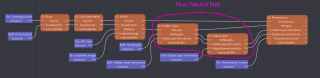
The neural network weights are 93KB of floats, and come into the shader as an SRV buffer NN Weights in the diagram above. Hidden Layer Activations is a buffer that holds 30 floats — one for each hidden layer neuron. Output Layer Activations is a buffer that holds 10 floats — one for each output layer neuron.
Below is the whole compute shader which evaluates the hidden layer. It’s very fast, but could probably be sped up by using group shared memory or actual matrix multiplies.
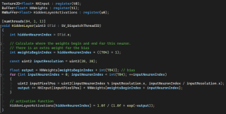
Evaluating the hidden layer.
When running the demo on an RTX 3090, the entire render graph executes in about half a millisecond, with the neural network part coming in at only 283 microseconds. The important takeaway here is that while training can take a long time, using the resulting network (inference) can be very fast. The training can be a tool time operation, much like baking lighting. And if you’ve ever baked lighting, you’ll know that while it can take a frustrating amount of time, it’s not a runtime cost. You just don’t want to “rebake” frequently.
Now let’s take a look at the demo below.
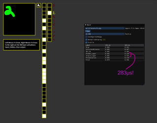
To the right of the green drawing area, you’ll see a small number 2. This is the input layer of the network arranged into a 28x28 image. To the right of that drawing area are 30 boxes stacked in a vertical line. These are the hidden layer neurons where black is 0, white is 1, and gray is somewhere in between. All of these went through a sigmoid activation function, so they’re conveniently tone-mapped to the display!
To the right of our hidden layer neuron boxes are our output layer neurons boxes. As you can see, the largest value (brightest white) is the value that is lit up in yellow.
This technique is fast, but it is still only a single invocation of a neural network. If we wanted to run a neural network per pixel, this network would be out of budget, even if we ran it at a smaller resolution. Doing per-pixel neural network operations thus presents us with a challenge: making a network that is small enough to fit in memory and perf budgets, but still large enough to be useful.
Other Information and Observations
Neural Network Alternatives
Neural networks can find solutions to problems where no good algorithm is yet known, such as machine vision or language tasks. However, not all problems are best solved by a chain of matrix multiplies (or convolutions for CNNs), interleaved with nonlinear functions.
At SIGGRAPH 2023, there was a paper that was competitive with all other NeRF papers, but didn’t use neural networks. Gradient descent was used to adjust 3D gaussian splats in world space to match photographs of a 3D scene, reconstructing the original scene to render novel viewpoints. Besides training quickly, the splats can be rasterized pretty efficiently, making it render in real time. They do take up quite a bit of memory though. You can find more details — plus some traditional game dev compression tricks — at https://aras-p.info/blog/2023/09/13/Making-Gaussian-Splats-smaller/
Training as a Process
There are several works of research that try to break open the black box of successful neural networks and try to understand what was learned. One paper talks about how to convert a neural network to a decision tree.
While training our network on MNIST only took 90 seconds, standard training can take days or weeks, even with a cluster of high-end computers! The good news is that because game development teams often already have both a light baking process and a cluster of machines with nice GPUs, the same setups can be used for ML training. The bad news is they would then be competing for the same resources!
Deep Learning
Have you heard the term “deep learning” come up in discussions around ML?
From the 1980s until the 2000s, we were in an “AI Winter” where machine learning faced a plateau of advancement it couldn’t overcome. One of the problems was that if you had too many layers in a network, the gradients would go to zero (vanishing gradients) or infinity (exploding gradients). “Deep Learning” was the term used to describe the goal of training a deep neural network with many layers. Researchers finally achieved this by changing how training worked, using different activation functions and different network architectures to allow derivatives to make it through deeper networks.
Conclusions
If you’ve made it this far, congratulations!
You should now have a solid understanding of the basics of machine learning and differentiable programming, and should be able to start experimenting with them on your own.
You may also be wondering if using plain C++ to do machine learning is a good idea or not. As far as training goes, it probably would make most sense to go with something like pytorch or similar and use the “industry standard” tools. Going this route would give you access to the latest and greatest algorithms and allow you to more easily find people to help you when you get stuck or run into problems. It’s also easier to hire for.
Runtime is a different story though. There are inference libraries and middleware to do inference in C++, but these tend not to be appropriate for use by game dev out of the box. In game development, we need to use our own allocators, we usually need exceptions turned off, we need to manage our own threads, we would prefer not to use the STL, we have sub-millisecond budgets, and so on. These requirements are not common outside of game development, and game developers don’t make up the largest group of coders out there, so the best practice at the moment seems to be to roll our own runtime inference.
NVIDIA did recently release differentiable slang, however. Slang is an HLSL+ shader language which can be compiled down to plain HLSL and other shader languages. The differentiable portion also survives this transformation. Differentiable slang opens the door to doing learning — not just inference — at runtime on the GPU, in DX12, Vulkan, and even consoles.
Further Reading
Want to continue exploring gradient descent and machine learning topics? Here are a few breadcrumbs to follow as you continue on your journey:
- Adam - An improvement to vanilla gradient descent. https://www.geeksforgeeks.org/intuition-of-adam-optimizer/
- Other activation functions like relu (https://www.tensorflow.org/api_docs/python/tf/keras/activations/relu) or selu (https://www.tensorflow.org/api_docs/python/tf/keras/activations/selu).
- Convolutional Neural Networks. (https://www.mathworks.com/videos/introduction-to-deep-learning-what-are-convolutional-neural-networks--1489512765771.html)
- Variational auto encoders - useful for data compression, denoising, and more! https://www.techtarget.com/searchenterpriseai/definition/variational-autoencoder-VAE
- NeRFS - they combine neural networks and ray marching! https://www.youtube.com/watch?v=CRlN-cYFxTk
- Instant NGP - a runtime friendly NeRF that can also be used as generic data storage. https://www.youtube.com/watch?v=A2FpIsfl8Nc
- Diffusion https://www.youtube.com/watch?v=1CIpzeNxIhU
- Cifar-10 data set (labeled small color images) https://www.cs.toronto.edu/~kriz/cifar.html
